Saint-Venant solver
How to use
It is important to use small enough space step. In the validation example 7 m was used. The SV model works with Chézy friction. It accepts Manning as input, and then it converts it to Chézy. From this constant Chézy value the friction coefficient Cf is calculated at every timestep. If given initial profile is used, it should also be coming from a profile calculated with Chézy.
Example
An example:
%Input variables

SimTime=13500; %in seconds
s=0.0015;
L=7000;
Bw=3;
z=0;
n=0.03;
dt=10;
SimLength=floor(SimTime/dt)+1;
qu=ones(1,SimLength+1)*1.5;
qd=ones(1,SimLength+1)*1.5;
qu(2:floor(3600/dt))=3;
q=1.5;
h=3;
NodeNum=1000;
HinitGiven=0;
UseInitialization=0;

[ Time,Hm2 , ~,~] = FiniteVoumeModel11bck(L, z,Bw,n,s,SimTime,dt,qu,qd,h,NodeNum,UseInitialization, HinitGiven );
 plot(Time,Hm2(:,end),'--r')
Initialisation module
An initialisation module can be called:
[ Time,Hm2 , Hm,HinitH] = InitialiseFiniteVolume(L, z,Bw,n,s,SimTime,dt,qu,qd,h,NodeNum )
When steady state initialisation is used, sometimes there is a very little bump /valley due to the different friction treatment. This function runs loops, so that the starting water depth is really the desired one.
Validation
Steady state validation
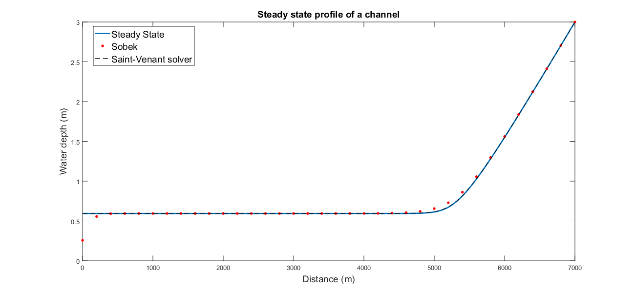
The steady state profile calculated by Sobek is compared to the one calculated by the steady state and also the result of the SV solver. The following data was used: s=0.0015; L=7000; Bw=3; z=0; n=0.03; q=1.5; h=3;
For the SV: dt=10 NodeNum=1000
The Sobek results are obtained with 200 m spatial discretisation and 5 min timestep, and 33.333 Chézy value. Note that the first two values of the Sobek results are different due to the location of water level and velocity nodes.. Note for the Sobek comparison that the value of the first two nodes is a bit different. No similar issue is noticed downstream. Another practical note: if you copy a Sobek model, usually you just need the .dsproj file. However, when a “hot start” is used, then the initialisation file is needed. It is a zip file, located in the dsproj folder.
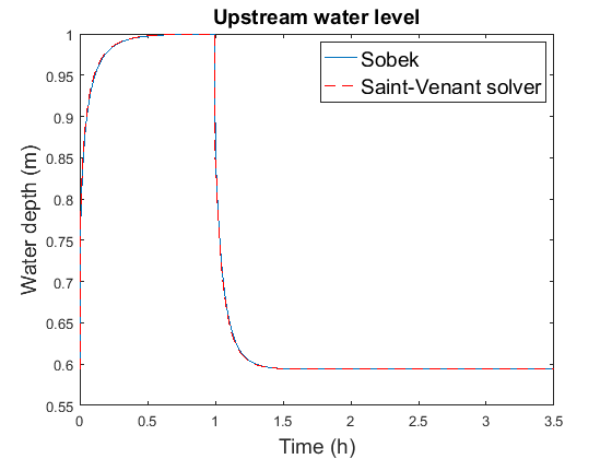
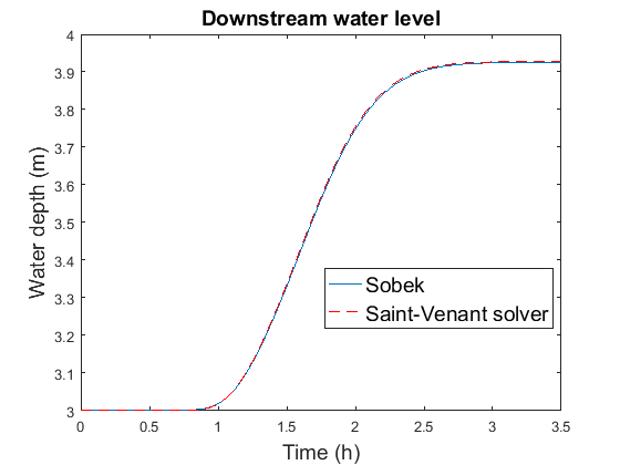
Unsteady state validation
A step response is compared. The following data is used:
SimTime=13500; s=0.0015; L=7000; Bw=3; z=0; n=0.03; dt=10; q=1.5; h=3; NodeNum=1000; HinitGiven=0; UseInitialization=0;
The upstream step is 1h long and the discharge increases to 3 m3/s. The same discretisation is used for Sobek. For the comparison for the upstream the second node is used.
Implementation
Explicit.
To do
- The downstream water level (or even structure) boundary condition should be checked.
- Revise the comments
- Revise the boundary conditions
- Document the trapezoidal validation